

FAQs
Videos
The MV5 and the ML5 can be purchased with either the J1939 or the CANopen communication option.
Yes, we have mounted a downloadable STP (STEP) file on the Documentation tab of this product web page.
If you are using SensorConnect:
- Launch SensorConnect and connect to the inertial sensor as normal.
- Click Save/Load Settings.
- Click Load Factory Default Settings and a confirmation message box appears.
- Click Load and the message box disappears. A green notification message appears in the upper right corner of the screen to indicate success.
The inertial sensor is now set to the factory default settings.
If you are using MIP Monitor:
- Launch MIP Monitor and connect to the inertial sensor as normal.
- Click Settings.
- Click Load Default Settings and a confirming message box appears.
- Click OK and the message box disappears.
The inertial sensor is now set to the factory default settings.
Yes, the inertial sensor does have a specialized mini DB9 connector which supports power, communication, and PPS functions. We recommend that you consider using our model 6224-0100 Craft Cable to make your own customized connections. This ‘craft’ cable has the mini DB9 on one end and 9 each 18-inch color-coded flying leads on the other. With this flexibility you can craft any power and/or communication and/or PPS configuration that suits by applying your own connectors, power sources, lengths, etc. Click here for a link to the craft cable mechanical drawing.
Yes, we have mounted a downloadable STP (STEP) file on the Documentation tab of this product web page.
Although the inertial sensor’s magnetometer is calibrated at the factory to remove any internal magnetic influences in the device, measurements are still subject to influence from external magnetic anomalies when the sensor is installed. These anomalies are divided into two classes: hard iron offsets and soft iron distortions. Hard iron offsets are created by objects that produce a magnetic field. Soft iron distortions are considered deflections or alterations in the existing magnetic field. Ideally, these influences are mitigated by installing the sensor away from magnetic sources, such as coils, magnets, and ferrous metal structures and mounting hardware. However, often these sources are hard to avoid or are hidden. To mitigate this effect when using the magnetometer to aid in heading estimations, a field calibration of the magnetometer after final installation is highly recommended.
All of the filters mentioned above are “estimation filters” (EF). When talking about estimation filters, one can quickly get mired in alphabet soup.
A Kalman Filter (KF) is a linear quadratic estimation algorithm that operates recursively on noisy data and produces an estimate of a system’s current state that is statistically more precise than what a single measurement could produce.
An Extended Kalman Filter (EKF) is used generically to describe any estimation filter based on the Kalman Filter model that can handle non-linear elements. Almost all inertial estimation filters are fundamentally EKFs.
An Adaptive Kalman Filter (AKF), technically speaking, is also an EKF but it contains a high dependency on “adaptive” elements. “Adaptive” technology refers to the ability of a filter to selectively trust a given measurement more or less based on a “trust” threshold when compared to another measurement that is used as a reference. The 3DM GX4-25 and -15 rely on adaptive control elements to improve their estimations and hence we refer to the estimation filter used in those devices as an “AKF”. Technically speaking it is an “EKF with heavy reliance on adaptive elements” or possibly an “Adaptive Extended Kalman Filter”. We just call it an AKF.
An Auto-Adaptive Extended Kalman Filter (AA EKF) is an adaptive EKF that, like the AKF described above, has “adaptive” elements that selectively trust given measurements more or less based on comparison to reference inputs. The difference with the auto-adaptive filter is that the “trust” thresholds are automatically determined by the filter itself. The filter collects error metrics on all the measurements and uses this to determine appropriate trust thresholds. This feature makes tuning a Kalman Filter for optimum performance much easier than manually determining these thresholds. The GX5/CX5/CV5 series introduces the Auto-Adaptive feature whereas the GX4 series has fixed adaptive thresholds.
A Complementary Filter (CF) is commonly used as a term for an algorithm that combines the readings from multiple sensors to produce a solution. These filters usually contain simple filtering elements to smooth out the effects of sensor over-ranging or anomalies in the magnetic field.
The 3DM-CX5-45, 3DM-CX5-25, and 3DM-CX5-15 support two communication interfaces:
- USB2.0 (full speed), and
- TTL serial (3.0 VDC, 9,600 bps to 921,600 bps, default 115,200 bps).
The 3DM-CX5-10 supports:
- TTL serial (3.0 VDC, 9,600 bps to 921,600 bps, default 115,200 bps).
The 3DM-CV5-25 and 3DM-CV5-15 support two communication interfaces:
- USB2.0 (full speed), and
- TTL serial (3.0 VDC, 9,600 bps to 921,600 bps, default 115,200 bps).
The 3DM-CV5-10 supports:
- TTL serial (3.0 VDC, 9,600 bps to 921,600 bps, default 115,200 bps).
This inertial sensor supports both RS-232 and USB 2.0 communications out-of-the-box.
The inertial sensor can communicate with the host computer by either connecting our model 6212-1000 RS-232 cable or our model 6212-1040 USB cable.